Simulating the Double Pendulum

An Introduction to Numerical Modeling II

Introduction

In the previous activity, we modeled a bouncing ball with Python. There, we focused our efforts mainly on writing an energy conserving update scheme that evolved the ball forward in time. In this activity, we will sharpen other Python skills that will be useful in numerical modeling. To do this, we will be modeling the double pendulum.

The double pendulum is an extension of the simple pendulum. The double pendulum we'll be simulating consists of one pendulum with a bob attached to its end and attached to this bob is a second bob on a second pendulum, see the image below. We won't derive the equations of motion for this system here (the Wikipedia article goes into more detail for those interested). The trajectory of the double pendulum is very different from the simple pendulum. Predicting the motion solely form the initial configuration is very difficult and in most cases impossible. This sensitivity to initial conditions tells us that the double pendulum is a system which exhibits chaotic motion. We will try to get a feel for the motion of the double pendulum by numerically modeling it and animating its motion.

For this activity we'll be focusing on two pieces of the Python code, the Bob Class and the plotting functions. Before we dive into the code, remember to use all available resources if you get stuck with any Python syntax. Some good resources are Google, the Python documentation and the Codecademy glossary.

Download the code and open it in your Python environment. Give it a quick read through and identify where the "Fix me!" lines are. The structure of this program is the same as the bouncing ball program. You'll notice that we aren't using our update_leapfrog function from that activity. Instead we'll be using one of SciPy's integration packages, odeint.

Classes in Python

Classes are Python's implementation of Object-Orientated Programming. They allow programmers to "bundle up" related variables and functions into one overarching object. The class we'll be working with contains all of the information of each bob at the end of a pendulum. We'll call it the Bob class. The Bob class holds the position, velocity, mass and rod length of each pendulum.

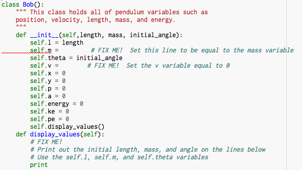
Go to the top of the program and look for the definition of the Bob class. Notice that there are several "Fix Me!" lines that need to be fixed. Here we're just setting some of the variables inside the Bob class to the user defined values. Follow the example of completed lines to fill in the missing code in the Bob class.

Once we've initialized our pendulum, we want it to print out its properties. We can do this by calling the display_values function that is inside the Bob class. Complete the print statement inside the display_values function so that it displays the pendulum's length, mass, and initial angle.

Now that our Bob class is complete we can move on to plotting.

Plotting in Python

One of the main advantages of using Python for scientific computing is its plotting library, matplotlib. This allows you to quickly and easily view your data in many different ways. For our double pendulum simulator, we'll be using the plot function. This function is the general plotting function for Python. It takes a list of x-values and a list of y-values as inputs and produces a graph of the data.

In the function initialize_plots(), find the first line that has a "FIX ME!". It should look like this,

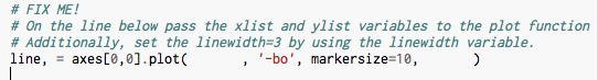
Once this line is fixed, it should plot the double pendulum as three connected points. Right now, the plot function isn't plotting anything. Plot the xlist and ylist variables by inserting them into the blank space after plot( . Look at the examples of the other plot functions for guidance.

Additionally, we want the line that connects the points to be thick. We can tell the plot function to do this by passing it the keyword argument, linewidth. Set the linewidth equal to 3 in the final blank space of the plot function. As an example, look at how we set the markersize variable to 10.

The Simulation

Now that we've completed our program, we can run our model of the double pendulum. The idea is the same as for the bouncing ball model: we numerically integrate the equations of motion and display the results.

To load in all of the functions hit the Run button in Canopy. If you had errors in the lines you fixed, you'll have to go back and fix them before you can run the model. If your script loaded without errors, then call the evolve function to start the simulation. The evolve function takes the initial lengths, masses, and angles of the two bobs.

Reproducing the simple pendulum

To check that our model makes sense in the case of a simple pendulum, call the evolve function with the second mass set to zero, evolve( 1 , 1 , 1 , 0 , 0.6, 0, 25, 0.1). Your output should look similar to this,

The top left plot shows us the pendulum in real space.

The top right plot shows us the pendulum in what is called phase space. Instead of plotting the x,y coordinates of the bob, we plot its angular velocity versus its angle from the vertical. This plot will give us an idea about how chaotic the motion is. Qualitatively, if there is no discernable pattern in the top left plot, we can guess that the motion is chaotic. Notice that for the blue points, the motion is clearly not chaotic as these points always lie in an oval.

The bottom left plot shows the angle of each bob as a function of time. We see a clearly oscillatory pattern.

Finally, the bottom right plot shows the total energy of the system (magenta line) and the energies of each bob. Remember that the total energy of the system should remain the same at all times.

The double pendulum

Let's test out another configuration, but this time we'll make the bobs of equal mass. Call the evolve function with the same arguments as before, but change the mass of the second bob to 1, evolve( 1 , 1 , 1 , 1 , 0.6, 0, 25, 0.1). What has changed? What effect did increasing the mass of the second bob have? Make a prediction for what will happen when you continue to increase the mass of the second bob. Test your prediction by calling the evolve function with the mass of the second bob equal to 10, and then equal to 100. Was your prediction correct?

The inverted pendulum

Let's look at the case of the inverted pendulum, i.e a pendulum where the bobs are at the top rather than at the bottom. The inverted pendulum is an example of an unstable equilibrium where the slightest nudge will send it swinging down. Call the evolve function again but this time set the initial angles of the two bobs so that they are at the top. Your output should look similar to this,

How does this motion compare with the cases from before? How would you describe the motion of the red bob?

Let the experiments begin!

Now that you've got a feel for how to use the model. Try out different configurations and see how regular or periodic the motion is. Try varying the lengths of the pendula or their starting angles.

If you want to do more coding, try changing the color of the lines and the size of the bobs in the plots. A more challenging exercise would be to convert the program into a collection of classes, i.e take all of the simulation functions and put them into a Simulation class.