How to make a ball bounce with Python

An Introduction to Numerical Modeling

Introduction

In this activity we will explore how to use Python to solve the equations of motion for a ball thrown off of a ledge. You should have some experience with Python syntax at this point, but feel free to use Google, the Python documentation , or the Codecademy glossary to refresh your memory.

For those with a lot of Python experience, there are some challenges at the end of the activity that should be more than enough to do.

A simple solver

Before we start coding, let’s get familiar with how we can solve for the position and velocity of our ball as a function of time. The idea is to use the definitions of position, velocity, and acceleration that involve a small time interval, \(\Delta t\).

$$ v = \frac{\Delta x}{\Delta t}$$ $$ a = \frac{\Delta v}{\Delta t}$$ For our freely-falling ball, \( a = - 9.8 \, \text{m} \, \text{s}^{-2} \). Given the initial position and the initial velocity, we can solve for the change in position and velocity over the time interval \(\Delta t\). $$ \Delta x = v \Delta t $$ $$ \Delta v = a \Delta t $$ Let \(x_i\) and \(v_i\) be the initial position and velocity and \(x_f\) and \(v_f\) denote the position and velocity after the time interval \(\Delta t\). We can use the above equations, and \(\Delta x = x_f - x_i\), \(\Delta v = v_f - v_i\), to solve for \(x_f\) and \(v_f\). $$x_f = x_i + v_i \Delta t$$ $$v_f = v_i + a \Delta t$$ Here we made the assumption that the acceleration is constant and that \(v=v_i\) in the update equation for the position. We will see later whether or not this is a good assumption.

Let’s start coding

You will be filling in some missing code in the Python file, bouncing_ball.py . To download the file, either click it or right click it and select Save Link As. This should download the program with the .py extension. Open up the file by double clicking it. The Canopy Python environment should open up and you should see the code in the Editor window. Here's what you should see if you sucessfully downloaded and opened the file,

Take a look at the different functions, their comments, and overall structure of the program. The main functions that we’ll be dealing with are the update functions and the evolve function. The flow of the program looks like this,

The entry point for the program is the evolve function. This function takes the initial velocity, height of the ball, and increment in time, \(\Delta t\). With these initial conditions, it sets the initial position and velocity of the ball (in two dimensions), sets up the plotting environment, and starts the main loop that advances the ball forward in time.

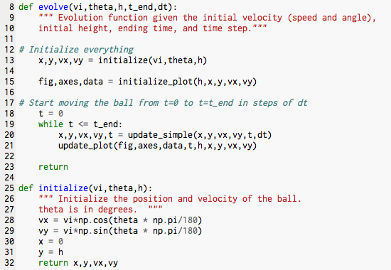
As our first task, we need to complete the missing pieces of the update_simple function.

Fill in the missing pieces of the update_simple function where there is the comment # FIX ME! . Use the update equations for \(x_f\) and \(v_f\) from above. What is the acceleration in the x and y directions? Also be sure to increment the time by \(\Delta t\)!

Once you’ve filled in the missing pieces for the update_simple function. Hit the Run button in the toolbar above the editor. This will run the code in the editor window and allow you to access all of the functions in the Python terminal. Now call the evolve function with the arguments evolve( 5, 15, 10, 30, 0.1). What do these arguments represent?

If you filled in the missing code properly, you should see a window pop up with four plots.

• The top left plot shows an animation of the ball bouncing.
• The top right plot shows the x and y velocities of the ball over time.
• The bottom left plot shows the x and y positions of the ball over time.
• The bottom right plot shows the kinetic and potential energies of the ball over time.

Does anything strange or unphysical happen to the ball as it bounces? Look at both the ball bouncing as well as the energy plots. What should be happening? At the end of the simulation your plot should look like this,

An energy conserving update scheme

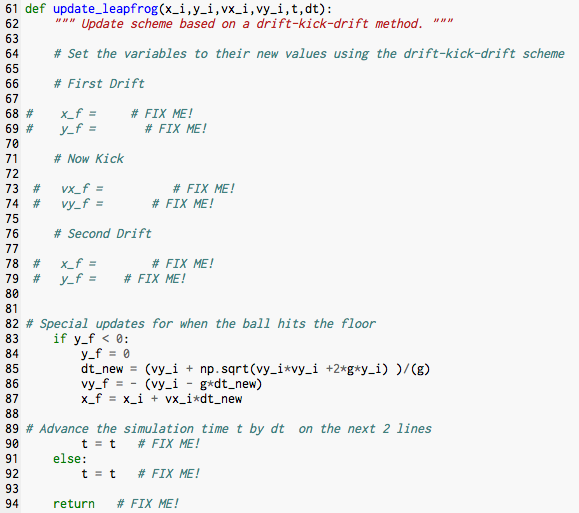
The problem with our simple update algorithm from above is that it does not conserve energy. We would like to create an update scheme that conserves the ball's energy at all times. To do this we can use what is called a drift-kick-drift (DKD) scheme (also called the Leapfrog method or the Velocity-Verlet method). The algorithm is split up into three steps,

• Drift: Slide the particle at its current velocity for a half time interval, \(\Delta t/2\).
• Kick: Give the particle a “kick” in velocity by accelerating it for a full time interval, \(\Delta t\).
• Drift: Slide the particle again at its new velocity for a half time interval, \(\Delta t/2\).

Translate these three steps into update equations and code them up in the missing lines of the update_leapfrog function. Don't forget to update the time and return the new positions and velocities! Before you start writing code, write down the algebraic equations for x_f and v_f in the same way as we did before.

In the evolve function, modify the line which calls the update_simple function to call the new update_leapfrog function . Hit the Run button again to load all of the changes you’ve made. Now evolve the system by calling the evolve function with the same input values as before, evolve( 5, 15, 10, 30, 0.1). Look at the energy plot as the ball bounces. Have we fixed the problem of energy conservation? Your final plot should look like this,

Run the evolve function for five different combinations of initial speed and direction. Save the final images using the save button on the plotting window (the "floppy disk" image).

Challenge: Making our ball more realistic

Now that we have a ball that can bounce perfectly elastically, let’s add in some inelasticity into our ball. When a real ball bounces, it deforms slightly. When it deforms it heats up due to friction and the energy that went into the heat is lost forever. This suggests that the kinetic energy in the ball before it bounces is greater than the kinetic energy in the ball after it bounces. We can parametrize this with the coefficient of restitution. This coefficient is a number between 0 and 1 that relates the y-velocity of the ball before it bounces to the y-velocity of the ball after it bounces. A coefficient of restitution equal to 1 implies that the ball is perfectly elastic and that there is no deformation of the ball as it bounces. A coefficient of 0 implies that the ball sticks to the ground completely and doesn’t bounce at all.

Add a new function called update_dissipative to the program. This function should be the same as the update_leapfrog function except in the lines of code that handle the ball bouncing. Define a new variable that holds the value of the coefficient of restitution and modify the new y-velocity that the ball has after the bounce to include the effect of deformation discussed above.

Be sure to evolve your squishy bouncing ball by calling the update_dissipative function inside the evolve function and see if it behaves as you would expect.

More advanced material

Here are some things to try if you breezed through the activity.

1. Take a look at the plotting functions and try to understand how Python plotting works if you’ve never done it before.
   
   
   • Try to plot another quantity in one of the plots.
   • Change the color and width of the lines.
   • Change what shape the points are.
   • Add in more background details in the top left plot.


2. Modify the program so that it uses Python Classes. Make a ball class that has x, y, vx, and vy attributes, and bounce and move methods.


3. How would you implement a wall to the right? Imagine the problem of throwing a ball against the wall. What if you also put in a wall to the left? Or someone that could catch the ball if it’s at the right height?


4. Add in air resistance or spin (one is much more difficult than the other!).


5. Make the acceleration due to gravity a function of the height of the ball. Imagine throwing the ball from the Moon.


6. Modify the program to use one of Python's differential equation solvers. For example the odeint integrator from the SciPy library.


7. Was the coding style of this program different than your own?

Some concluding remarks

Hopefully by the end of this activity you have a better idea about how to solve the equations of motion of an object numerically using Python. The basic idea was to take small steps in time and then change the objects position and velocity by using their definitions as rate of change quantities (i.e \( v = \frac{\Delta x}{\Delta t}\)).

Additionally, we validated our program by relying on simple physical principles such as energy conservation. This is a key thing to remember when coding up solutions to physics problems. Your program may not crash but the output may not make sense physically. It's always important to test your program versus known physics; this is how we know we did the programming correctly!

I'd also encourage you to try out the ideas laid out in the advanced material section. Even if you do only one a day, or one a week, they will provide extra practice with programming in Python, and also extra practice in doing physics.