(Re)Discovering Dark Energy and the Expanding Universe: Fitting Data with Python

Introduction

Through observations of the local and distance Universe, astronomers have determined that our Universe is made up of three types of matter and energy:

1. ~30% Matter. This includes regular matter ( ~4%) like you and me and also Dark Matter (~26%). Dark matter is inferred through the gravitational influence of “invisible matter”. That is, we see the influence of matter through gravity, but we don’t see any matter.
2. ~ 0.01% Radiation. This is mostly the cosmic background radiation.
3. ~70% Dark Energy. Dark energy makes up 70% of the “stuff” in our Universe and supplies the energy that drives the expansion (and acceleration) of the Universe.
4. In addition to matter and energy, the Universe is also measured to be flat. This has important implications for the evolution of the Universe.

It is still unknown what exactly Dark Energy is, but the evidence for it is very convincing. To measure Dark Energy, astronomers need to observe distant galaxies and measure how far away from us they are and how fast they are moving away from us. That is, astronomers need two independent measurements of as many galaxies as possible, distance and velocity away from us.

First, to measure the distance, astronomers observe a special class of supernovae. The Type Ia Supernova (SnIa) is special because astronomers know the intrinsic brightness of all SnIa. The Type Ia is a powerful and important example of a standard candle in astronomy. If we know how bright an object actually is, then we will know its observed brightness (the thing we measure with telescopes) if it is placed at any distance from us.

Second, to know how fast a galaxy is moving away from us we can use the Doppler Effect. Astronomers measure the spectrum of a galaxy (or the SnIa) and look for redshifts in the emission lines. The more shifted a line in the spectrum is towards the red, the faster that galaxy is moving away from us. The amount by which an emission line is shifted into the red is termed redshift. For close-by galaxies the redshift is directly proportional to its recessional velocity.

If we can measure both the redshifts and the distances to many galaxies, then we can better understand the evolution of our Universe.

As we will see in this activity, our Universe is expanding. In fact, it is not only expanding but doing so at an accelerated rate. The unknown mechanism that causes this observed accelerated expansion rate we call Dark Energy.

The Data

For this activity we will be using real data from a group lead by the Nobel Prize winner Adam Riess. His team measured the distances and redshifts to hundreds of galaxies by observing these Type Ia Supernovae. We will be using that same data to discover Dark Energy.

The supernovae data are in the file sn_data.txt. Each line in the file represents one galaxy and it consists of three columns. The first column is the redshift to the galaxy (i.e how fast its moving away from us), the second is the distance (in Mpc) to the galaxy, and the third column is the error in that distance measurement.

We will be using Python to do our data analysis. With the numerical (Numpy) and scientific (Scipy) libraries, plotting and fitting the supernovae data will be a breeze.

As always, remember to use all available resources if you get stuck with any Python syntax. Some good resources are Google, the Python documentation and the Codecademy glossary.

Python

The Python code for this activity is split into two files. The linear fit script is here , and the quadratic fit script is here. Download both of these and open them up in the Canopy editor.

To fit the supernovae data, we will be using the Scipy function curve_fit(func, x,y). This will fit the x,y data to the function func. If we have information about the errors in x or y, we can pass these to curve_fit to get an idea about the errors in the fitted parameters.

Part one will focus on fitting a linear relationship between supernova distance and redshift. Part two will fit a quadratic relationship between supernova distance and redshift.

Hubble's Law

Open up the linear_fit.py script and read over the comments and code. The script loads the data by opening the sndata.txt file and then fits the data to a linear function given by,

distance = 300,000 * redshift / H

Where H is an unknown parameter. Astronomers call H the Hubble constant after Edwin Hubble. When we fit the data to this linear relationship we are determining what value of the Hubble constant best fits the data. The current value of the Hubble constant is roughly between 60 and 70 (the difference depends on the type of data collected). The Hubble constant tells us two important things.

1. The inverse of H gives us the age of the Universe.
2. It allows us to connect redshift with distance through the fitting function above (Hubble's Law). That is, if we measure a redshift, then using Hubble’s Law, we can convert this into a distance.

Find all of the FIX ME!s in the script and fix them by following the comments. Once you've fixed all of the missing code, run the file by pressing the green play button at the top of the editor. If you made the correct fixes, you should see a plot pop up that shows the supernovae data, as well as the best fit line to that data. In the console at the bottom you should also see a print out of the results, giving you the value and error on the best fit value of H. Does this look like a good fit to the data? Your plot should look something like this,

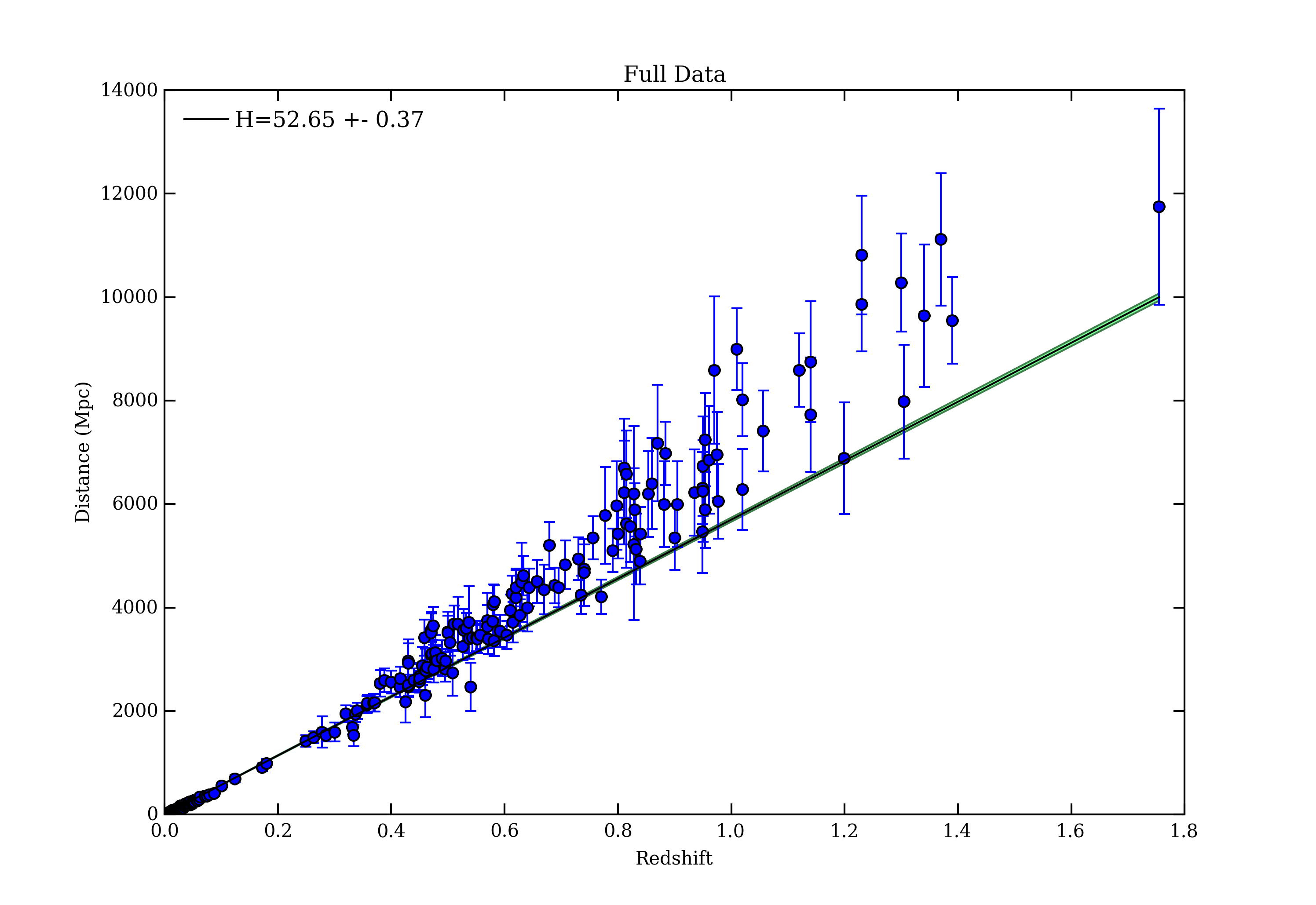
The green band around the best fit line shows the spread in our fit based on the spread in the fitted value of the Hubble Constant.

An approximation

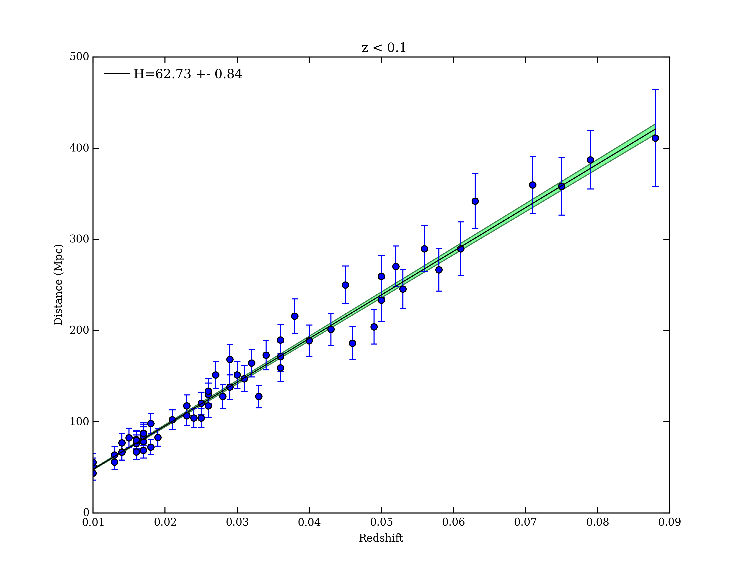
Hubble’s Law is really only valid at very small redshifts. Try fitting the data again with the same fitting function but this time only fit a small subset of the data. Uncomment the bottom lines of the linear_fit.py script and fix the remaining missing pieces of code and rerun the script by hitting the green play button at the top. This time you should see a second plot pop up that shows only the data with redshift less than 0.1. How does this value of the Hubble constant compare with the best estimates to date (use Google to find this)?

The Accelerating Universe

In the previous section we found that a linear relation between redshift and distance was not good enough to fit the full domain of observed supernovae data. We can go one step further and add a quadratic term to the fitting function. This introduces a new parameter that is historically called the deceleration parameter q. If q is non-zero and negative this suggests that the further away a galaxy is from us, the faster it is receding from us. Our fitting function is now,

distance = 300,000 * ( redshift + 0.5 * (1 - q) * redshift^2 ) / H

Note that we now have two parameters, H and q.

Open up the quadratic_fit.py file to fit the data to this new quadratic function. The beginning of the script is the same as the linear_fit.py script. Go through and fix all of the FIX ME!s and read all of the comments. Once you've fixed all of the missing code you should have a plot which shows you the best fit curve to a subset of the supernova data. What are the values of H and q when you fit supernovae with redshifts less than 0.5? Your results should look similar to this,

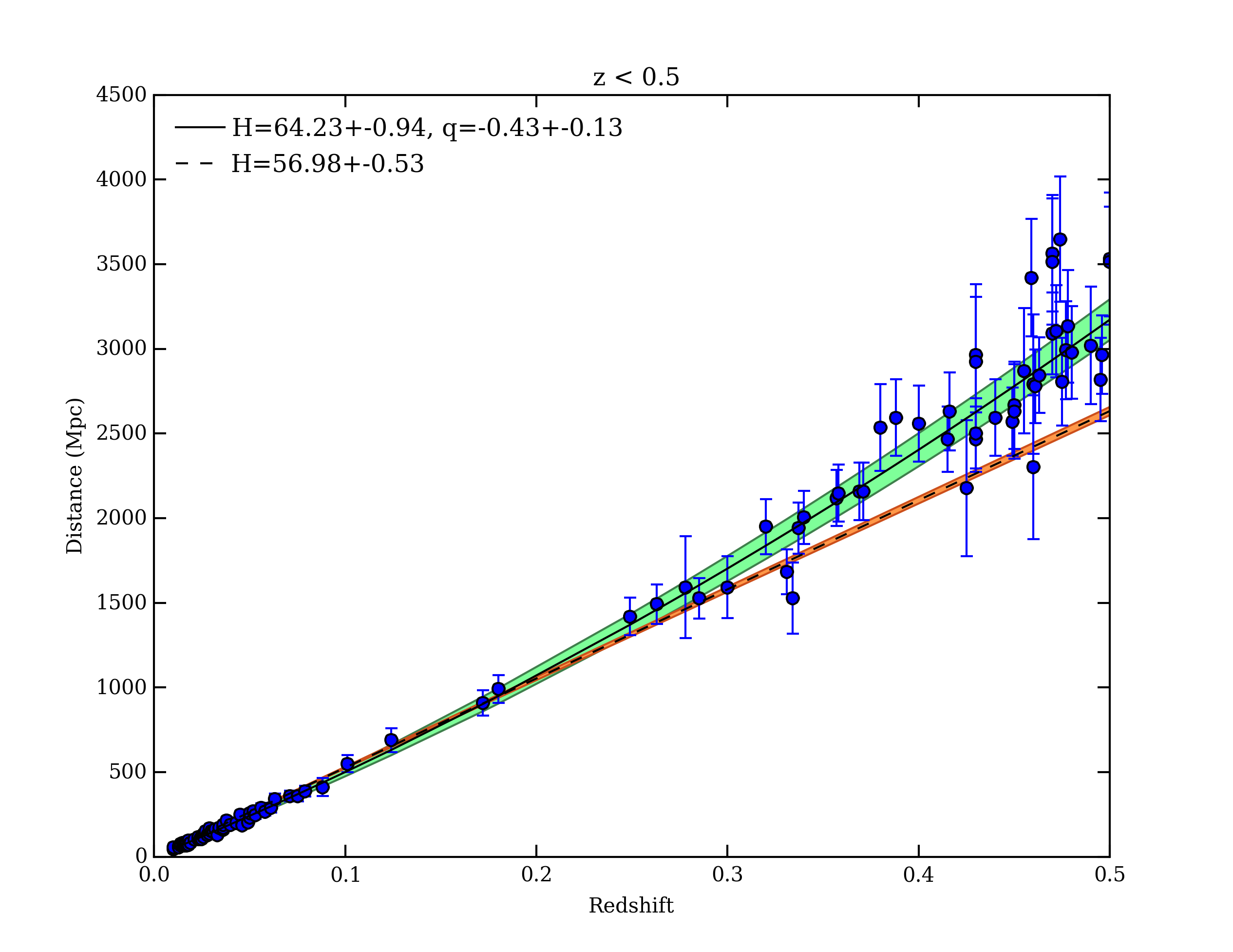
If your best fit q is negative, then congratulations you just discovered Dark Energy and the accelerating Universe! Try rerunning your script with different values of zmax to fit different subsets of the data. What zmax gives the best fit by eye? Can you come up with a quantitative test to determine the best value of zmax to use? Try making a new plot that shows the values of q and H as functions of zmax.

Notice that we still haven’t got a good fit to the data at redshift greater than one. In reality the fitting function is much more complicated and can’t be written as a simple polynomial. But for small redshifts it can be approximated by one, as we’ve just seen.

Extras

Some extra things to do if you've discovered Dark Energy are:

• Fit the data to a cubic polynomial by replacing q with q + a*x. The new parameter a tells us how the deceleration parameter varies with redshift.
• Combine the two scripts into one unifed framework of functions and classes that will fit the supernovae data and present the results.
• Use the chi_squared function at the top of the script to calculate how good of a fit you have. The lower the value the better the fit. Use this to make a plot of chi_squared versus zmax to determine the best value of zmax to use.